In Praise of Shadows and Light: Climate-Resilient Passive Solar Design for University Buildings

孟子程 · 郑达均 · 周方亚诺

2026 MCM/ICM · Problem E

Summary

As climate change intensifies the frequency of extreme weather events, the design of climate-resilient architecture becomes imperative. Passive solar strategies offer a sustainable pathway to decarbonization, yet their effectiveness varies drastically across climatic zones. This study constructs a comprehensive mathematical framework to optimize passive design, transitioning from single-building retrofits to global generalizability and future-proof construction.

For Model 1, addressing the cooling-dominated context of Sungrove University (25.8°N), we formulate a Dynamic Thermal Balance Model (DTBM) coupled with Monte Carlo optimization to identify effective retrofit strategies. By rigorously computing hourly unshaded fractions for rectangular and arc-shaped shading, we identify Scheme A (Rectangular Overhang) as the superior solution. The optimal design achieves a 46.9% reduction in annual cooling load (91,323 kWh saved) while maintaining visual comfort, demonstrating that geometric simplicity can yield substantial thermodynamic benefits in subtropical climates.

For Model 2, extending the framework to the heating-dominated Borealis University (60°N), we integrate high-capacity thermal mass and dual-setpoint heating into the DTBM. The analysis reveals a critical trade-off: while passive strategies reduce annual heating energy by 65.3%, the requirement for rapid morning warmup in high-mass structures causes an increase in peak power demand. This finding highlights the physical limitation of purely passive solutions in sub-arctic regions, suggesting that energy savings must be balanced against grid capacity constraints.

For Model 3, evaluating the generalizability of these strategies, we conduct a sensitivity analysis across 30 locations spanning latitudes 15°S to 75°N. Spearman rank correlation analysis identifies universal design principles: thermal mass requirements scale exponentially with heating dominance (p = +0.807), while envelope insulation must be coordinated with solar altitude rather than temperature alone. Crucially, we find that optimal Solar Heat Gain Coefficient (SHGC) is constrained primarily by comfort feasibility (0 = —0.498) rather than simple energy minimization.

For Model 4, synthesizing these insights for a new Student Union building, we implement a Two-Stage Multi-Start Stochastic Search to balance energy, glare, and daylighting under current and future (2040 SSP2-4.5) climate scenarios. The resulting holistic design reduces cooling loads by 60.4% in the 2040 scenario compared to a code-compliant baseline, while simultaneously reducing glare risk hours by 78%.

Overall, our framework provides a transferable, scientifically grounded methodology for climateresponsive design. By integrating precise geometric modeling with stochastic uncertainty analysis, we demonstrate that passive architecture can be both robust to future climate variability and adaptable to diverse geographic contexts.

Keywords: Dynamic Thermal Balance Model, Monte Carlo Optimization, Passive Solar Design, Climate-Resilient Architecture

1 Introduction

As climate change intensifies the frequency of heat waves and drives up global cooling energy demands, the design of climate-resilient architecture has become a critical imperative. Passive solar shading strategies offer a sustainable pathway to mitigate thermal loads[1], yet traditional design methods—often relying on static solar angles at solstices—fail to capture the dynamic trade-offs between summer cooling reduction and winter heat preservation. In this study, a comprehensive mathematical modeling framework is formulated to generate and optimize passive solar design strategies for two distinct climatic contexts: the cooling-dominated environment of Sungrove University and the heating-dominated environment of Borealis University.

The research task is structured into four progressive stages. First, we formulate a dynamic thermal model for Sungrove’s Academic Hall North to optimize retrofit parameters—including shading geometry, glazing properties, and envelope insulation—aiming to minimize academic-year cooling loads. Second, the model is extended to the high-latitude context of Borealis University, where the integration of thermal mass is analyzed as a critical variable for balancing winter heat retention with summer overheating prevention. Third, the generalizability of these strategies is evaluated by conducting a sensitivity analysis across a spectrum of latitudes, identifying design principles that transcend specific locations. Finally, these insights are synthesized to propose a holistic passive design for the new Student Union at Sungrove University, ensuring long-term performance under future climate scenarios.

1.1 Problem Statement

The core challenge involves transforming the energy profile of educational buildings through passive interventions. For Sungrove University (Case 1: Low-Latitude/Hot), the existing Academic Hall North—a 60m xX 24m rectangular structure—currently relies heavily on mechanical cooling. The objective is to identify an optimal set of retrofit measures that minimizes the net cooling energy demand while respecting thermal comfort constraints.

Conversely, for Borealis University (Case 2: High-Latitude/Cold), the challenge shifts to maximizing solar harvesting in a limited daylight environment while utilizing thermal mass to dampen temperature fluctuations.

Specifically, this paper addresses the following interrelated tasks:

1. Retrofit Optimization (Sungrove): Develop a physics-based simulation to identify the optimal configuration of shading devices and building envelope parameters that minimizes cooling load (Qcoo1) While accounting for winter solar penalty (Q solar,winter)- 2. Thermal Mass Integration (Borealis): Investigate the thermodynamic coupling between shading and internal thermal mass to reduce heating demands in a sub-arctic climate.

3. Generalizability Verification: Assess the transferability of the proposed models across different latitudes and heating/cooling load profiles through multi-location experiments.

4. Architectural Synthesis (Student Union): Propose a holistic passive design for the new Student Union, expanding the optimization to a multi-objective framework that balances energy efficiency, daylight availability, and glare control under future climate scenarios.

1.2 Methodology Overview

A multi-stage simulation-optimization approach is adopted. The foundation is a Dynamic Thermal Balance Model (DTBM) that couples solar irradiance decomposition with a lumped-capacitance thermal network. The model is able to compute:

• Solar Geometry: Exact solar position and unshaded fraction (funshadea) for complex shading morphologies (Rectangular and Arc-shaped) at hourly intervals.

• Sol-air Temperature: The equivalent exterior temperature accounting for solar absorption on opaque envelopes.

• Thermal Dynamics: The time-evolution of indoor temperature (7;,) governed by envelope conduction, ventilation, and internal gains.

Optimization is executed via stochastic search strategies—specifically transitioning from global random sampling to a two-stage refinement protocol in complex scenarios—over a high-dimensional design space, incorporating variables such as shading projection (L), lateral extension (e), Solar Heat Gain Coefficient (SHGC), and ground reflectivity (p,), with additional parameters (e.g., thermal mass, orientation) introduced in subsequent models. To ensure scientific rigor, a Monte Carlo uncertainty analysis is integrated, perturbing meteorological inputs to construct confidence intervals for key performance indicators (KPIs), thereby quantifying the risk profile of the proposed designs. This paper focuses first on the detailed formulation and results for the Sungrove retrofit (Task 1), followed by the extensions to thermal mass and generalizability.

2 Assumptions and Notations

Modeling Assumptions To render the complex thermodynamic system tractable while maintaining predictive validity, the following assumptions are established:

• Lumped Capacitance Approximation: The building is modeled as a single thermal zone. This assumption is valid for comparative analysis of envelope performance, as high-level retrofit decisions (e.g., glazing type, shading depth) affect the global energy balance uniformly.

• Operational Consistency: HVAC systems typically operate via a deadband-controlled thermostat (Cooling: 24°C, Heating: 20°C) during occupied hours (08:00—18:00). However, specific models (e.g., Model 2) investigate dual-setpoint strategies with night setbacks to enhance energy conservation.

• Weather Data Strategy: Models 1-3 utilize clear-sky irradiance (Ineichen model[2]) and synthetic temperature profiles to isolate geometric design drivers. Model 4 advances this by integrating TMY and SSP2-4.5[3] future climate data to ensure robust performance under realistic and changing meteorological conditions.

• Decoupled Internal Loads: Internal heat gains are modeled as a constant flux during occupied hours, independent of the passive design features, isolating the impact of the retrofit variables.

Notation Summary Table 1 summarizes the primary variables, parameters, and symbols used throughout the model.

Table 1: Summary of primary notation used in the thermal model Symbol Description Units Typical Range L Shading overhang projection length m 0.10 — 2.50 e Shading lateral extension beyond window width m 0.00 — 2.00 SHGC Solar Heat Gain Coefficient - 0.15 —0.75 VT Visible Transmittance — 0.15 —0.75 Peg Ground reflectivity (albedo) - 0.05 — 0.80 UAeny Envelope thermal conductance W/K — 600 (baseline) m Ventilation mass flow rate kg/s_ 0.035 (baseline) Crone Zone effective thermal capacitance JK 2x 10°-10° Tin Indoor air temperature °C Tout Outdoor air temperature °C - Tair Direct normal irradiance Wim? lait Diffuse horizontal irradiance Wim — Tord Ground-reflected irradiance Wim? funshaded Fraction of window unshaded at time t - 0-1 Qcool Cooling load (thermal) kWh -— Qsolar,winter Winter solar heat gain kWh - Oheat Heating load (thermal) kWh — His Discomfort hours during work h - Agtare Glare risk hours h - Agaylignt Daylight insufficient hours h - Wj Weighting factors in objective functions - - WWR Window-to-Wall Ratio - 0.1 —0.7 Bouilding Building orientation relative to South deg -45-—+45 The academic year is defined from September | to May 31 of the following year, with a time step of one hour. Indices t denote discrete time steps, while subscripts s and n denote summer (June—August) and winter (December—February) periods respectively. The subscripts “base” and “cand” distinguish baseline and candidate designs in the objective function.

3 Model 1: Optimization of Retrofit Strategies for Sungrove University

This section addresses the specific requirements of Sungrove University, situated in a warm, lowlatitude climate where excess solar gain is the primary driver of energy consumption. The goal is to retrofit the existing Academic Hall North to minimize cooling loads (Q•oo;) without compromising visual comfort.

3.1 Proposed Shading Strategies

To minimize cooling loads while respecting architectural constraints, we specify two distinct shading typologies for evaluation. Scheme A (Rectangular Overhang) is a traditional horizontal overhang extending distance L from the wall, with an optional lateral extension e. This design is structurally simple and easy to retrofit. Scheme B (Arc-shaped Shading) is a complex geometry featuring a curved leading edge and extended side fins. This design is intended to better intercept low-angle sun (early morning/late afternoon) which simple overhangs often miss.

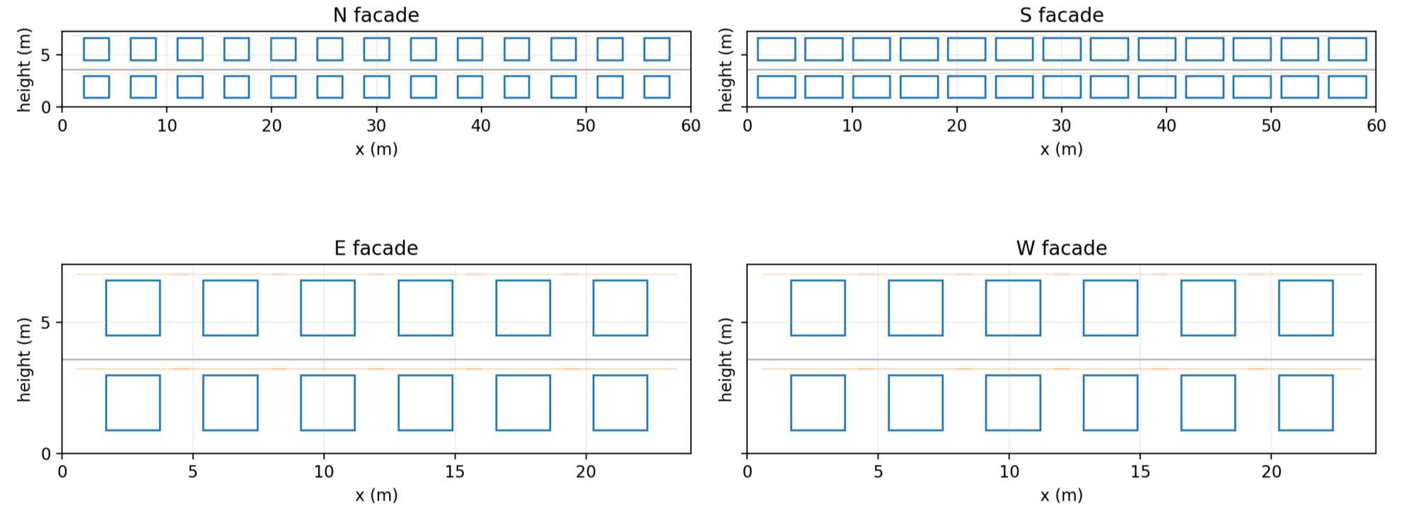
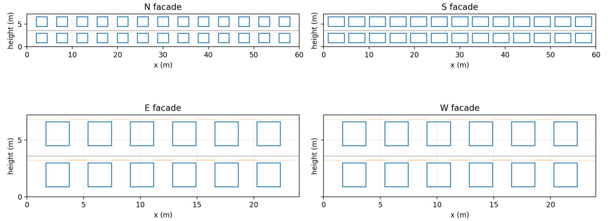
Figure 1 illustrates the baseline building compared to the optimized configurations (denoted as Scheme A* and Scheme B*) of these two proposed schemes. The specific optimization technique that we employed will be discussed later.

facade S facade facade S facade LP Dpoood Scccoon) oSSeScoeoesS E, cooogooo ooo OOOO LWCILICICICLILILI ? OOOO OOOOOoOoOoOD| sOoOooooOooooOoOoo ; ee See eee { SSS SSeS tra) 40 60 o 10 20 im 40 50 60 10 eon 5 60 i) 10 20 eo 40 50 60 E facade W facade E facade W facade H#LUUUOUUU|FJ,UUUUUU] ,OOOUOUO|JOOOUUO OOOOOOVOOUOOU OOOUOUUOUPVOOUOOUOo a 3 eS 20 i a” % 5 es 0 (a) Scheme A* (b) Scheme B* Figure 1: Visual comparison of the proposed shading strategies. (a) Scheme A* (Rectangular) offers deep overhead protection. (b) Scheme B* (Arc-shaped) wraps around window edges to block oblique solar angles.

3.2 Analysis and Modeling

To address the cooling load challenge at Sungrove University, we construct a Dynamic Thermal Balance Model (DTBM) coupled with a stochastic optimization engine. This framework mathematically quantifies the interaction between solar geometry, shading morphology, and building thermal inertia, enabling the identification of optimal retrofit parameters.

Solar Irradiance Decomposition and Vector Analysis The driving force of the thermal model is the precise decomposition of solar irradiance on vertical facades. For any given hour f, the sun’s position vector is defined by the altitude angle a(t) and azimuth A;(t). The angle of incidence 6(f) relative to a facade with surface azimuth @ is computed via spherical trigonometry[4]:

cos 6(t) = sina(t) cos B + cos a(t) sin B cos(A,;(t) — B) (1)

The total incident irradiance /;..(t) on the facade is synthesized from three components: direct beam Jgir, isotropic diffuse sky radiation Ig, and ground-reflected radiation Igrq.

Tgix(t) = max{0, DNI(t) cos 6(t) } (2a) Layn(t) = DHI(t) -~*S°5F (2b) Ipei(t) = pg GHI(1) - SF (2c)

Here, , (ground reflectivity) is treated as a decision variable, acknowledging that landscape modifications (e.g., paving materials, grass) can alter the thermal environment.

Algorithmic Shading Projection A distinct feature of this model is the dynamic computation of the unshaded fraction finshadea(t), Which governs direct solar ingress. Unlike static solstice-based methods, our algorithm integrates shading effects over the entire academic year. For Scheme A (Rectangular Overhang), the vertical projection angle (VPA) is derived from the solar profile angle: tan a(t) (3) cos AA(ft)

where AA(t) is the azimuth delta. The shadow depth is projected as S,4(t) = L- tan(VPA(t)). The unshaded fraction is then computed by intersecting the projected shadow polygon with the window geometry (Wwin, Hwin).

For Scheme B (Arc-shaped Shading), the projection length L(x) varies continuously along the window width. We employ a numerical integration approach, discretizing the window width into N segments and averaging the unshaded ratio for each segment to obtain an accurate scalar funshaded(f).

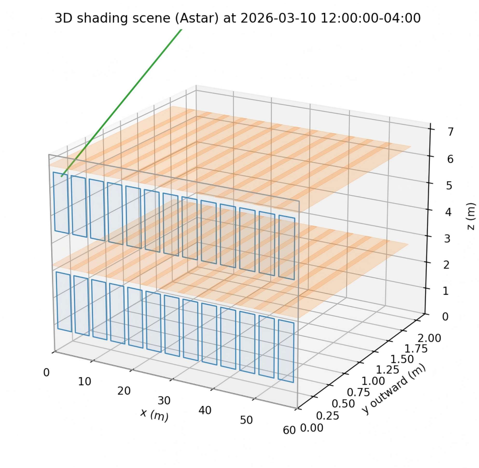
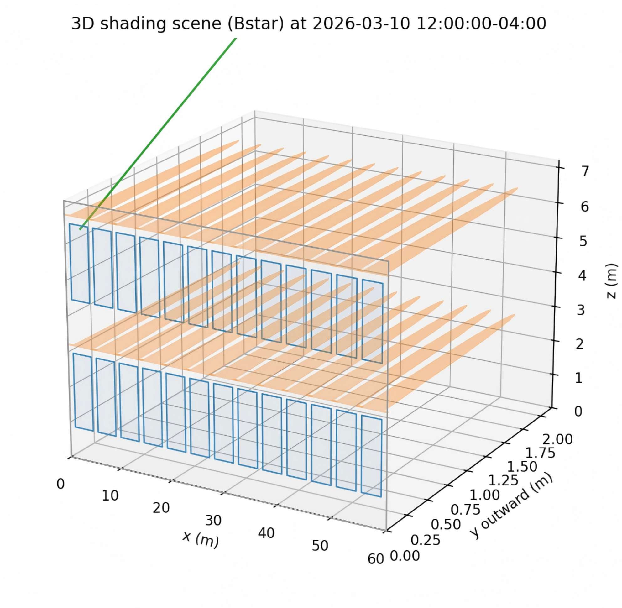
Figure 2 and Figure 3 show the 2D and 3D schematic diagrams of the optimal A/B projection, respectively. These diagrams provide an intuitive visualization of our shading projection algorithm.

tan(VPA(f)) = Shadow union example (Astar) at 2026-03-10 12:00:00-04:00 CODE Ee Ee Ce ee a LSE ES ES EE Ee es Ee Eee Ee TE 0 30 Al x along facade (m)

oN BO i) 60 (a) Scheme A*: 2D Projection Shadow union example (Bstar) at 2026-03-10 12:00:00-04:00 SN IN NN IN IN NN NN RE NN NN IN NN NN Ne Ne Ne 0 30 4 x along facade (m)

(b) Scheme B*: 2D Projection oN BOO of 60 Figure 2: 2D geometric validation of shadow coverage on the South facade (Solar Noon, March 10). The red regions indicate shadows cast by the overhangs; the blue rectangles are window modules. The overlap area is rigorously calculated to determine instantaneous solar gain.

3D shading scene (Astar) at 2026-03-10 12:00:00-04:00 3D shading scene (Bstar) at 2026-03-10 12:00:00-04:00 VA Ui fi 40 Mitr TRE oF NY Bu oo a z(m)

(a) Scheme A* (b) Scheme B* Figure 3: 3D visualization of the computed shadow cast for optimal Scheme A and Scheme B at solar noon, March 10. The algorithms precisely determine the unshaded window fraction (fiunshadeq) for every hour of the simulation.

Sol-air Temperature and Envelope Heat Transfer To account for solar absorption on opaque surfaces (brick veneer walls and roof) without modeling a full 3D conduction field, we utilize the Sol-air Temperature metric (Tgo-air)[5]._ This equivalent temperature linearizes the radiative heat balance:

Mab Tso1-air (t) = Tout (t) + z. . Leff opaque (t) (4) out where Jeff opaque 18 the area-weighted average irradiance incident on all opaque surfaces. This transformation allows the envelope heat gain Qeny to be computed as a simple conductive flux driven by the difference between T(o]-air and indoor temperature Tin:

Qeny(t) = UAeny - [ Tso1-air (t) 7 Tin(t)| (5)

Lumped-Capacitance State-Space Model The building’s thermal dynamics are governed by a first-order differential equation, discretized for hourly simulation. The indoor temperature state 7;, evolves according to the conservation of energy:

Tin (t + At) = Tin (t) At This formulation explicitly couples the thermal mass (Cz n-) with the instantaneous heat fluxes.

Crone = Qenv(t) + Ovent(t) + Osolar.in (t) + Oint(t) ~ Onvac(t) (6)

• Solar Gain: Qsolar.in (f) = Awin - SHGC - Sunshade (1) . I window (t)

* Ventilation: Qyen(t) accounts for both constant background ventilation and an optional Night Flush strategy, which activates enhanced airflow when Joy < Tin — AT, • during unoccupied nights to purge stored heat.

Optimization Problem Formulation The retrofit design is formulated as a constrained implementation of the global optimization problem. The specific objective function J maximizes the Net Energy Benefit, defined as the cooling savings minus a weighted penalty for winter heating loss:

max J (x) = (obese _ 2(%)cos1} —w- (Oe sinter - 2%) sola winter] (7)

The decision vector x = [L,e, SHGC, pg, UAscaie, Czone] spans the geometric and thermophysical design space. Constraints are imposed on thermal comfort, requiring the hours of discomfort (Hq) to remain below 400 hours/year.

The optimization is solved using a Random Search algorithm with Monte Carlo sampling (N=12,000)[6]. This method is chosen for its robustness in non-convex, discontinuous search spaces typical of building parameter optimization.

3.3. Results and Discussion The optimization identifies highly effective retrofit strategies for Sungrove University’s Academic Hall North. Table 2 summarizes the optimal design parameters and key performance indicators for both shading schemes compared to the baseline.

Table 2: Comparison of Optimal Retrofit Designs vs. Baseline Metric / Parameter Unit Baseline (NoShade) Scheme A* (Rectangular) Scheme B* (Arc) Design Parameters Shading Overhang (L) m - 1.91 2.34 Lateral Extension (e) m - 1.12 1.68 Glazing SHGC - 0.40 0.18 0.20 Ground Reflectivity (p,) - 0.20 0.05 0.12 Performance Indicators Annual Cooling Load kWh 171,876 91,323 94,817 Load Reduction To - 46.9% 44.8% Winter Solar Gain kWh 35,697 8,591 9,843 Net Benefit Objective kWh 0 51,242 49,364 Discomfort Hours h 161 123 167 Comparing the two optimized typologies, Scheme A* (Rectangular) outperforms Scheme B* (Arc-shaped) across most metrics. Scheme A achieves higher cooling load savings (46.9% vs 44.8%), lower discomfort hours (123 h vs 167 h), and has a lower estimated implementation cost ($80,216 vs $102,251 based on the linear cost model). The geometric simplicity of the rectangular overhang also implies easier constructability and maintenance. Therefore, Scheme A is recommended as the primary retrofit strategy for Academic Hall North.

Cooling Load Reduction and Energy Balance The proposed designs successfully address the primary challenge of reducing the academic year cooling load. Scheme A* achieves a 46.9% reduction in cooling energy demand (from 171,876 kWh to 91,323 kWh). This substantial saving is driven by a two-pronged strategy:

1. Deep Passive Shading: The optimal overhang length of 1.91 m significantly blocks high-angle summer sun.

2. High-Performance Glazing: The optimizer selected a low Solar Heat Gain Coefficient (SHGC ~ 0.18), indicating that preventing solar ingress is critical in this climate.

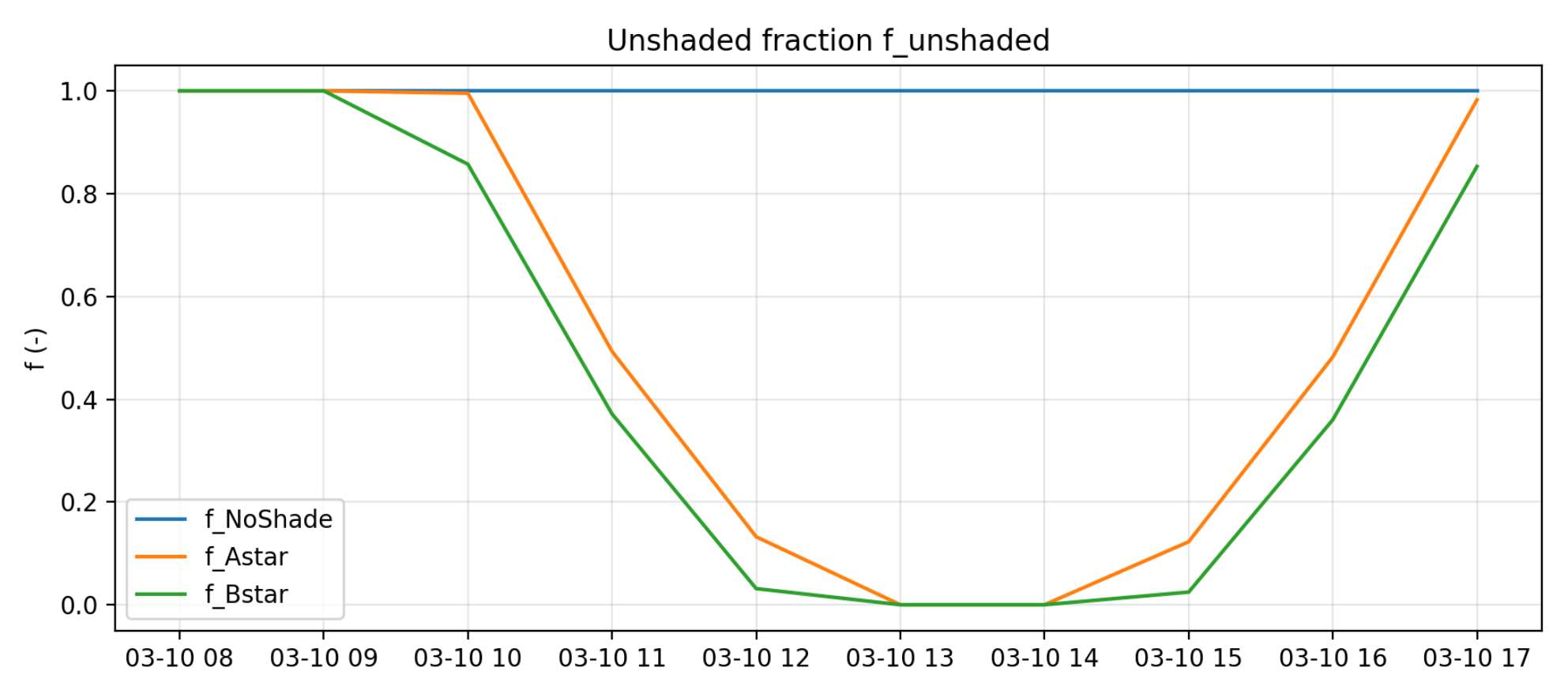
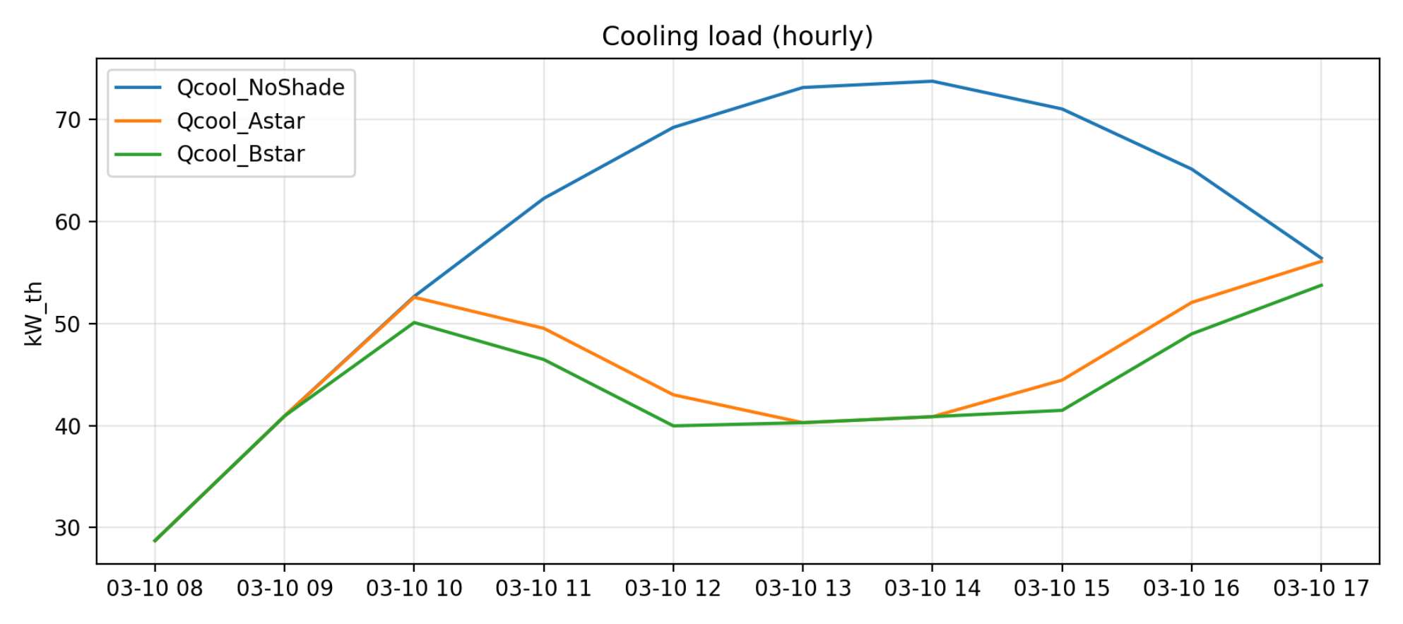
To visualize the dynamic impact of these strategies, Figure 4 presents the hourly performance for a representative spring day (March 10). The unshaded fraction profile (a) demonstrates how the optimized overhangs effectively truncate the solar window during high-intensity midday hours. Consequently, the cooling load profile (b) is significantly flattened, eliminating the sharp afternoon peak characteristic of the baseline building.

1.0 — Qcool_NoShade 70 Qcool_Astar os — Qcool_Bstar 60 0.6 — f NoShade f_Astar 0.04 — f.Bstar 30 kW_th w S 03-1008 03-1009 03-1010 03-1011 03-1012 03-1013 03-1014 03-1015 03-1016 03-1017 03-1008 03-1009 03-1010 03-1011 03-1012 03-1013 03-1014 03-1015 03-1016 03-1017 (a) Unshaded Fraction (funsnaded) (b) Cooling Load Profile (Q•oo1)

Figure 4: Hourly performance dynamics on March 10. (a) Schemes A* and B* maintain near-zero direct solar exposure during peak irradiance hours. (b) This geometric shielding results in a dramatic reduction in peak cooling demand compared to the unshaded baseline.

While the objective function includes a penalty for lost winter solar gain, the results show a trade-off: winter solar heat gain drops by approximately 76%. However, given Sungrove’s warm, cooling-dominated climate, this loss is acceptable as the reduction in cooling load (approx. 80,000 kWh) far outweighs the loss in winter gain (approx. 27,000 kWh), resulting in a substantial net positive energy balance. Furthermore, the problem statement highlights an issue with glare in the classrooms. While not explicitly part of the objective function, the shading design serves a dual function. By significantly reducing the unshaded fraction funshadea during work hours, the optimal overhangs naturally mitigate direct sunlight penetration, thereby alleviating visual discomfort and glare risks for students and faculty.

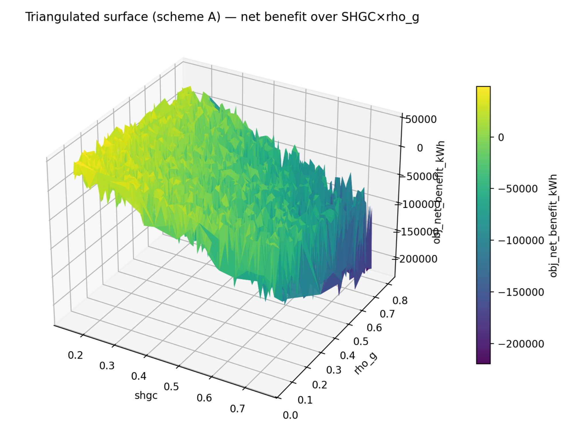
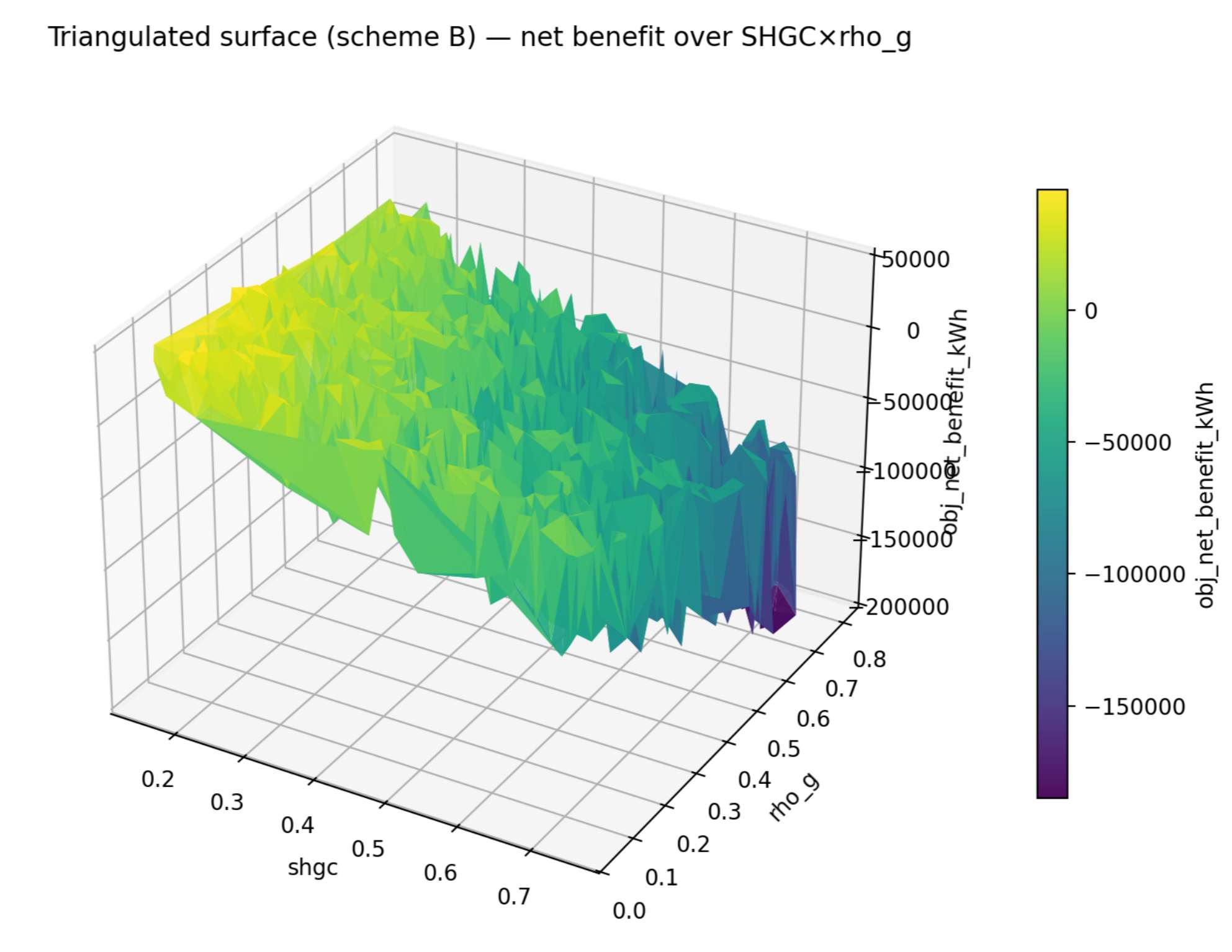
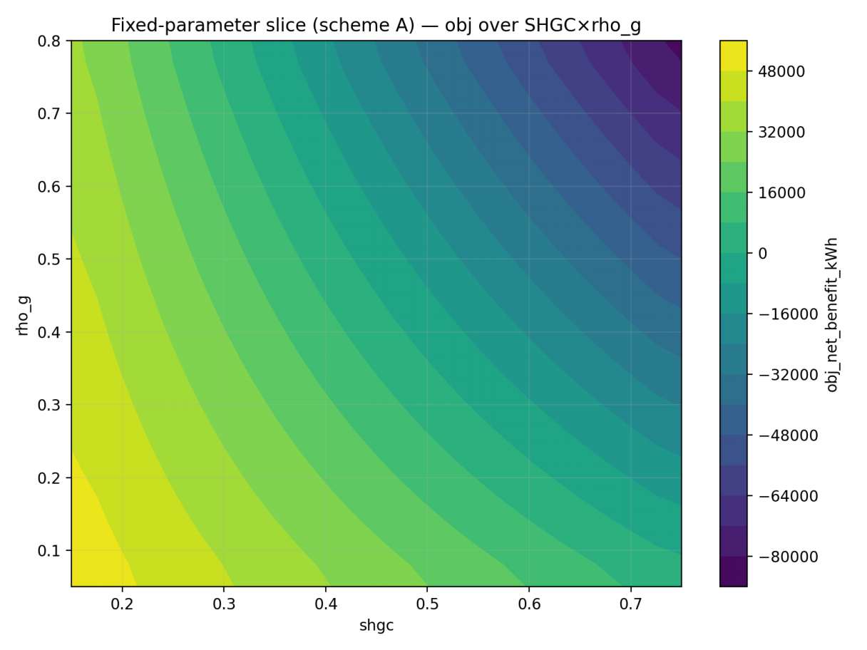
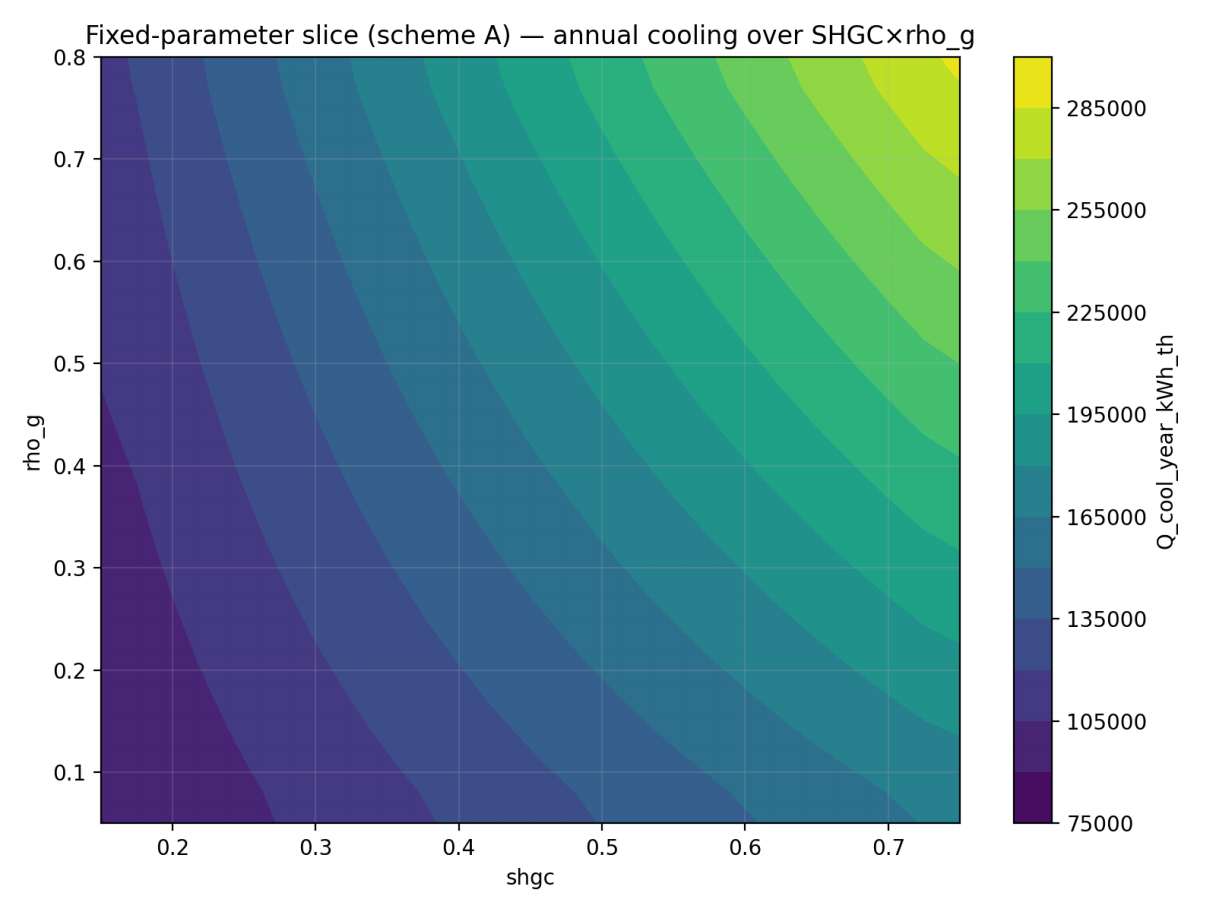
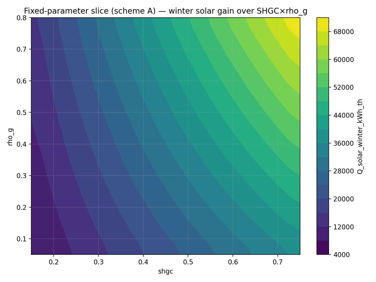
Parameter Sensitivity and Robustness Analysis Figure 5 presents the response surface of net benefit with respect to SHGC and p, for both schemes, showing lower SHGC generally yields higher net benefits in Sungrove’s cooling-dominated climate, while ground reflectivity exhibits more complex trade-offs. It decomposes the net benefit of A* into Triangulated surface (scheme A) — net benefit over SHGCxrho_g Triangulated surface (scheme B) — net benefit over SHGCxrho_g 0 0 c © -50000 = z 2! -50000 4! +7 oO 8 8 -100000 1! 2 2 2 5 100000 =! 3} o -150000 -150000 -200000 (a) Scheme A Surface Fi ‘heme A) — obj over SHGCxrho_g 285000 68000 0000 255000 $000 52000 225000 fit_kWh kWhth 44000 er_kWh_th 195000 *)

75000 02 03 oa 0s 06 o7 shoe 4000 (c) A*: Net Benefit (d) A*: Cooling Load (e) A*: Winter Gain Figure 5: (a)(b) show the response surface of Net Benefit (kWh) vs. SHGC and Ground Reflectivity (Pz) for Scheme A and B. (c) to (e) show the component decomposition of the objective function. The heatmaps illustrate the conflict between minimizing cooling load (darker is better) and maximizing winter gain (lighter is better), resulting in the net benefit topology.

annual cooling load and winter solar gain in the second row, revealing the dominant conflict: higher SHGC increases winter gain but penalizes cooling performance, with net benefit strongly driven by cooling reduction.

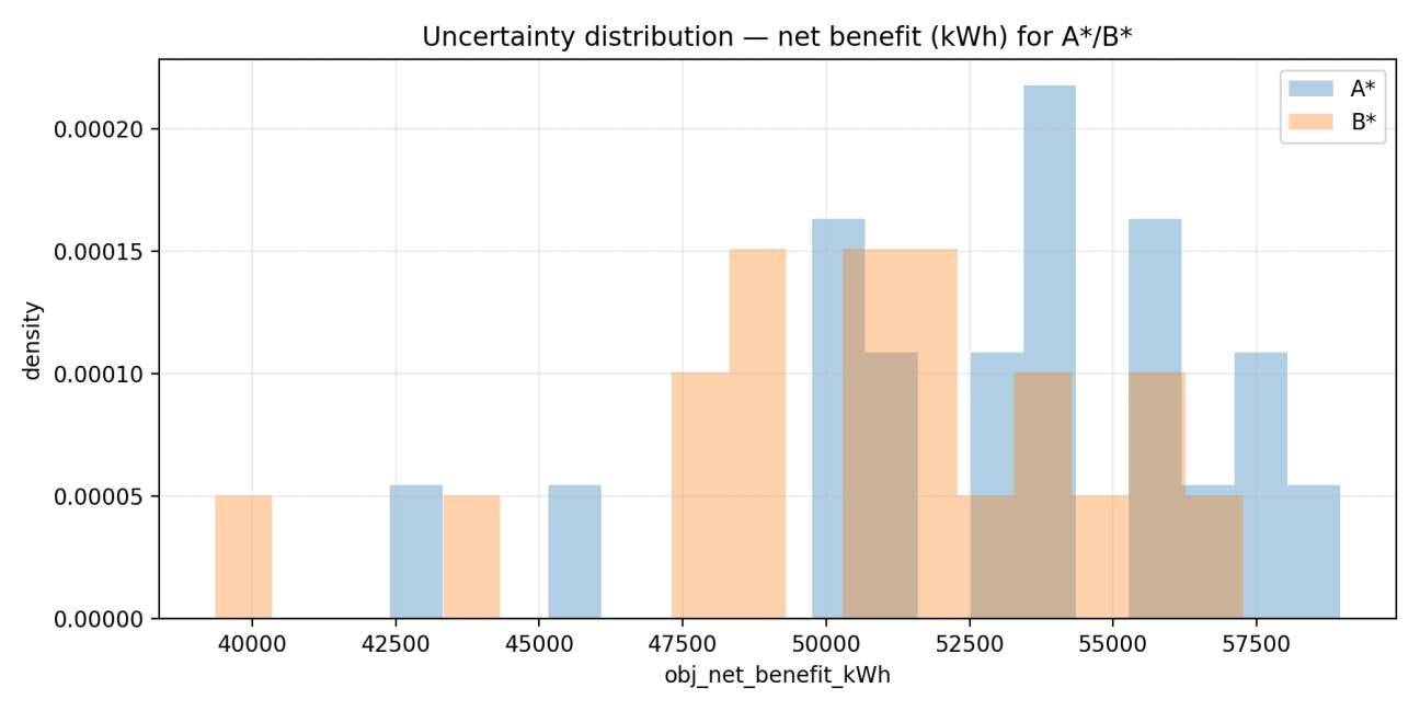
Uncertainty distribution — net benefit (kWh) for AY/B* Uncertainty distribution — annual cooling (kWh_th) Uncertainty distribution — discomfort hours (work time)

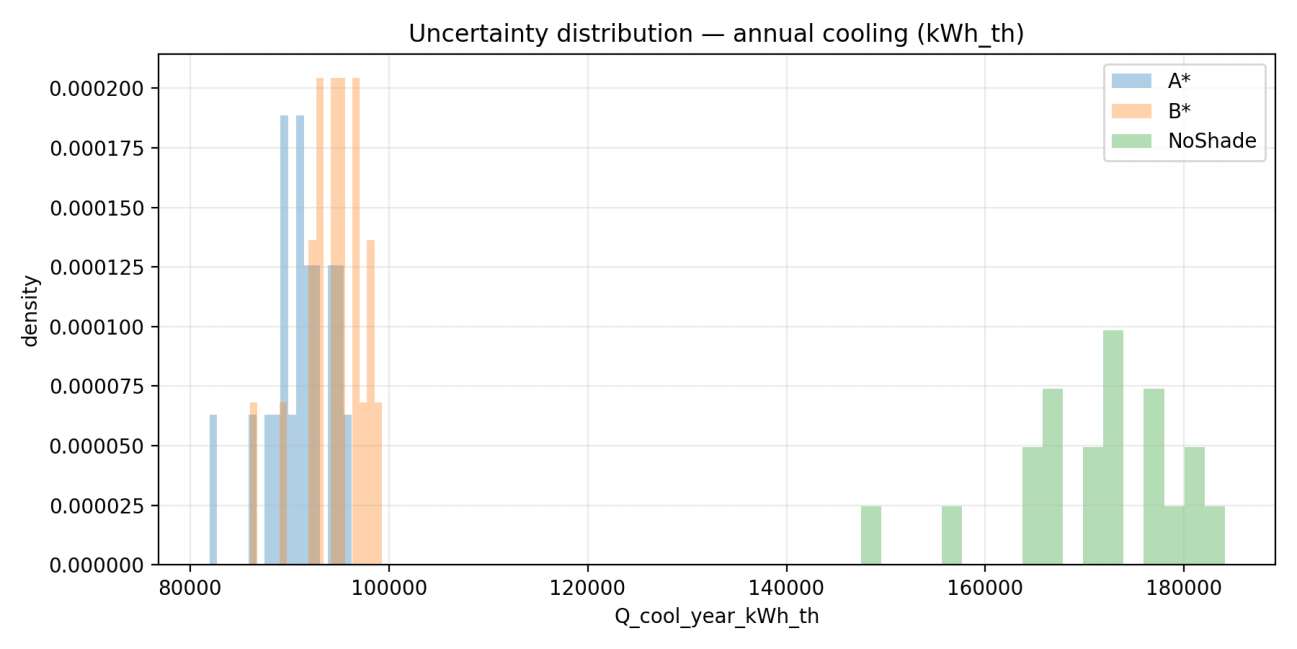
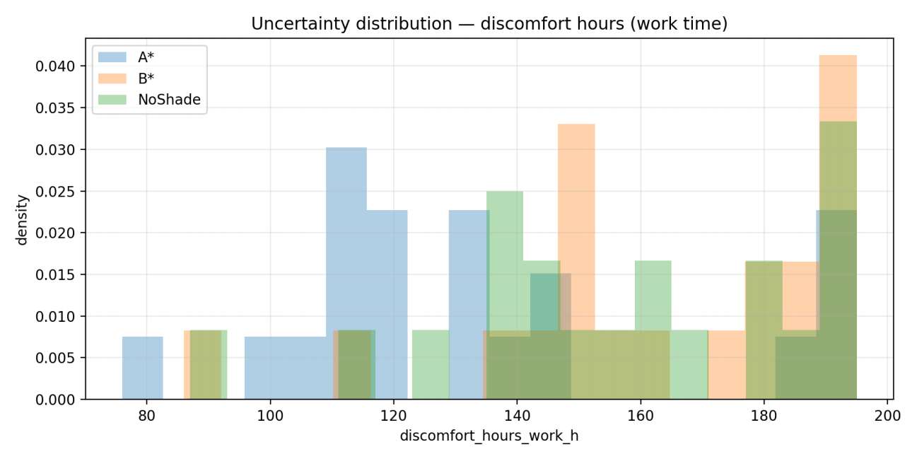
0.000200 = 0.040 ia 0.00020 a eo a Koos Noshade 03s] = Neshade 000150 0030 0.00015 o.000125 - . 0025 3 o.o0o10 4g 0.000100 $0020 0.000075 ons 0.00005 0.000050 ania o.0002s 0.005 a 40000 42500 45000 47500 50000 52500 55000 57500 80000 100000 120000 140000 160000 180000 - 00 120 140 160 180 200 bj. net_beneft kWh a kh 80 u -ool_year_kWh_th discomfort_hours, wor (a) Net Benefit Distribution (b) Cooling Load Distribution (c) Discomfort Hours Distribution Figure 6: Uncertainty analysis distributions for key performance indicators. The histograms show the frequency of outcomes across 20 Monte Carlo weather scenarios.

To assess robustness against climate variability, a Monte Carlo simulation with perturbed weather inputs was conducted. Figure 6 shows the resulting distributions for net benefit, annual cooling load, and discomfort hours. The optimal designs remain robust: for Scheme A*, the 95% confidence interval for annual cooling load is [83,956, 95,672] kWh, representing at least a 44% reduction versus the deterministic baseline (171,876 kWh) even under unfavorable conditions. Discomfort hours stay within acceptable limits in most scenarios. This confirms the long-term resilience of the design, ensuring significant energy savings and comfort protection under future climate variability.

4 Model 2: Thermal Mass Integration for Borealis University

This section addresses the design challenge for Borealis University (60°N), a heating-dominated sub-arctic climate where the primary objective shifts from cooling load minimization to heating load reduction while managing overheating risks during transitional seasons. We extend the Dynamic Thermal Balance Model (DTBM) with three critical enhancements: (1) thermal mass integration, (2) dual-setpoint heating, and (3) dynamic reflective blinds.

4.1 Climate Context and Baseline Issues

Borealis University presents a fundamentally different thermal challenge. With limited winter solar availability and low outdoor temperatures, passive solar harvesting becomes essential. However, baseline simulation reveals severe indoor overheating (peak temperatures exceeding 80°C, Table 3), indicating inadequate heat dissipation mechanisms during shoulder seasons.

4.2 Model Extensions Thermal Mass Dynamics

The extended state-space model explicitly incorporates thermal capacitance:

aT; . . . . . "= Qenv + Ovent + Osolar,in + Qint ~ Qheat (8)

zone “dt where Qnear represents HVAC heating power, and Czone (2x10 to 10 J/K) represents the combined heat storage capacity.

Dual-Setpoint Heating We implement dual-setpoint heating with night setback:

21°C. work hours (08:00—18:00) Tset (t) = (9)

17°C. non-work hours Dynamic Reflective Blinds Threshold-based reflective blinds activate during critical months (May-September):

0.25 if Iyindow(t) > 220 W/m? Tolinas(t) = aow(t) (10)

1.0 otherwise Parameter Adjustments Key adjustments from Q1 include a shift to latitude 60.17°N and longitude 24.94°E, with cooling disabled and heating operating continuously. Enhanced night flushing (0.5 kg/s) is introduced for heat dissipation, while the optimization uses 20,000 samples with penalty weights w; = 12 and w2 = 6 kWh/h.

4.3. Optimization Formulation The objective minimizes heating energy with comfort penalties: min J (x) = Onn" (x) + W 1 Hoverheat (X) + wW2Haiscom fort(X) ad 1)

where x = [L, e, SHGC, pg, UAscaie, Czone]- 4.4 Results and Analysis Table 3: Borealis University: Optimal Design Performance Metric Unit Baseline Scheme A* Scheme B* A(A) Design Parameters L (overhang) m - 2.40 2.02 - SHGC - 0.40 0.202 0.218 - Crone J/K 4x10’ 81x10® 95x 108 — Performance Indicators hows kWh = 33,670 11,700 13,800 -65.3% great kW 44.0 956 1,065 +2073% Hoverheat (work) h 1,217 683 566 —43.9% Evins kWh 742 4,543 4,857 +512% Ti" (work) °C 80.2 45.4 48.6 -—43.4% Key Findings 1. Heating Energy vs. Peak Power Trade-off: Scheme A* achieves 65.3% heating energy reduction but increases peak power by 2073%. Large thermal mass (Czone ~ 8 X 10° J/K) requires high instantaneous power for temperature setpoint changes.

2. Thermal Mass Dominance: Sensitivity analysis shows Czone aS most influential parameter (Spearman p = 0.83), strongly correlated with heating energy (po = -0.87) and peak power (p = 0.85).

3. SHGC Trade-offs: Optimal SHGC (0.202-0.218) balances winter solar gain (9 = 0.97) and overheating risk (9 = 0.55).

4. Geometric Patterns: Both schemes require substantial shading (L = 2.02-2.40 m). Scheme B needs full lateral coverage (e = 2.00 m) compared to Scheme A’s moderate extension (e = 1.28 m).

5. Comfort Limitations: Despite improvements, both designs exhibit substantial overheating (566-683 h) and discomfort (583-698 h), indicating inherent limitations without active cooling.

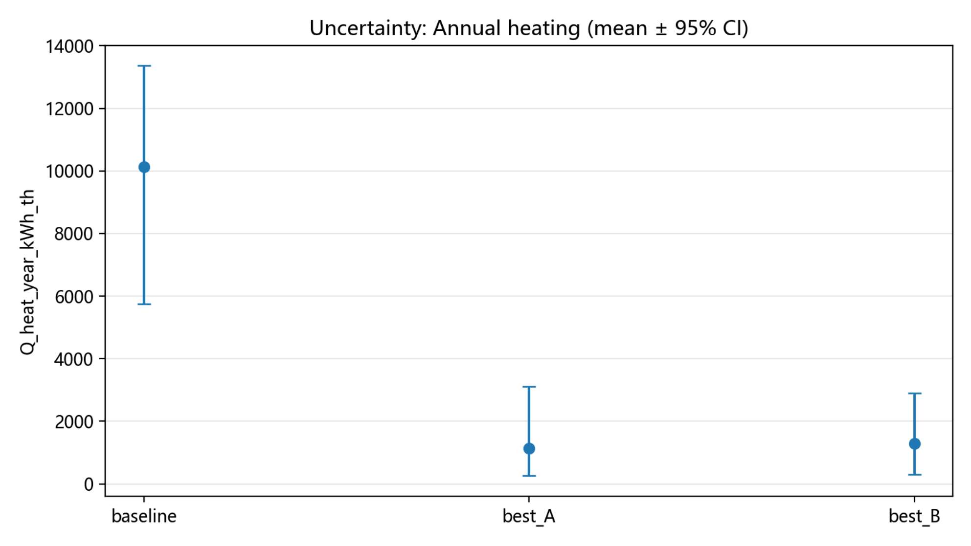
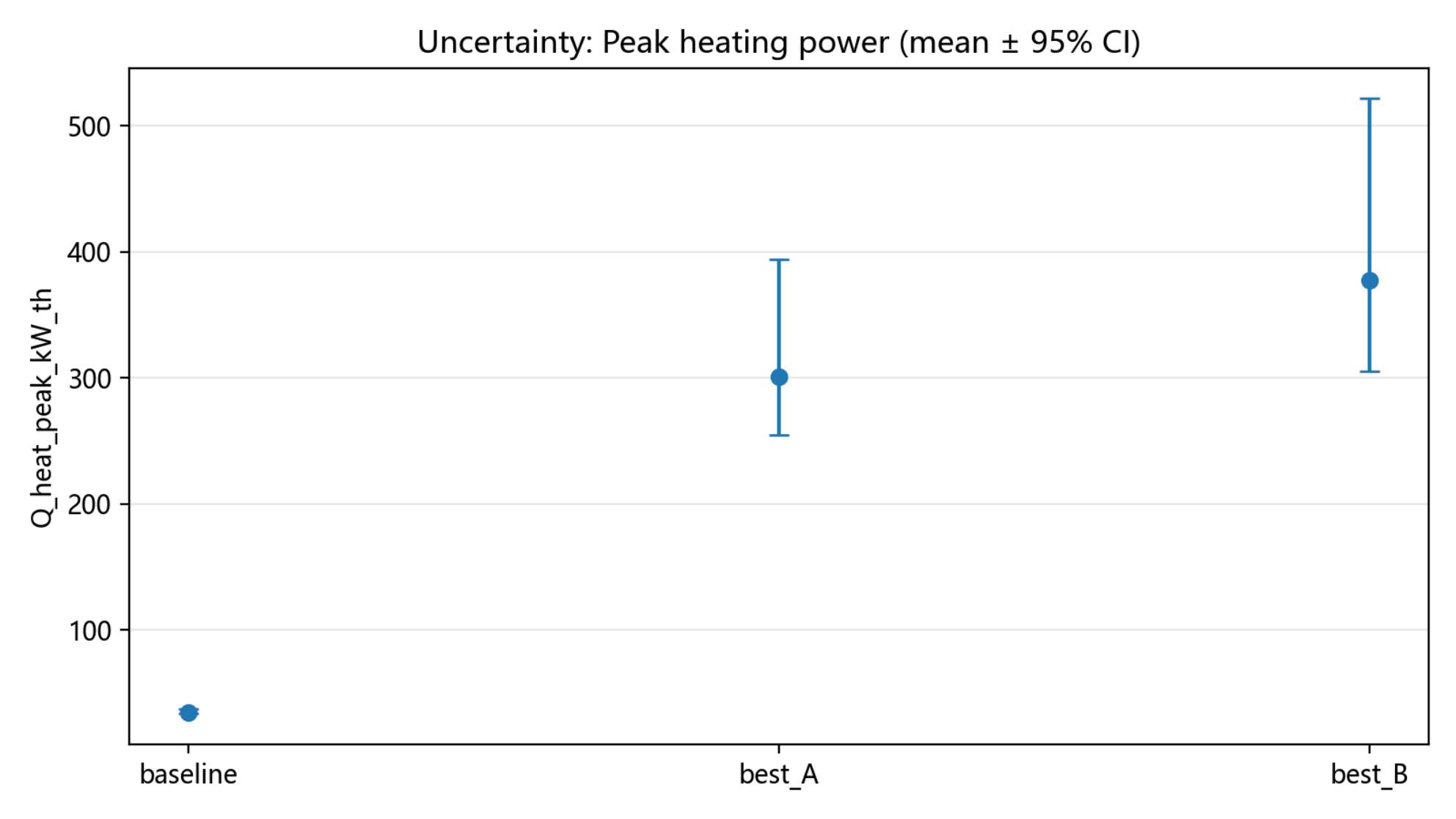
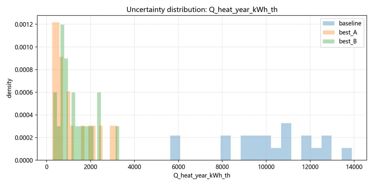
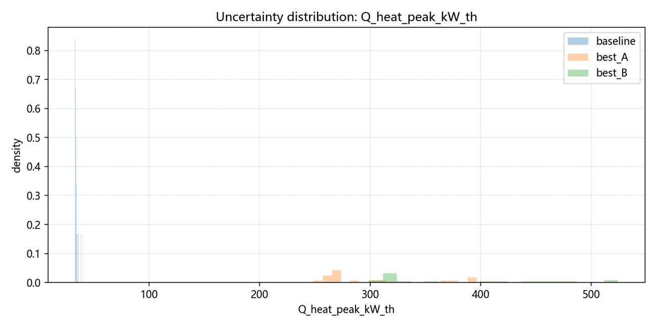
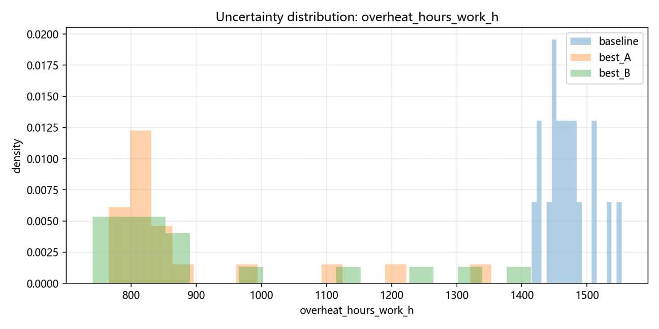
Uncertainty and Robustness Figure 7 shows 95% confidence intervals for key metrics across 20 weather scenarios. Heating energy savings remain robust across all scenarios, while peak power issues persist consistently. Figure 8 further confirms these trends, with clear separation between baseline and optimized heating energy distributions.

Uncertainty: Peak heating power (mean + 95% Cl) 14000 500 + 12000 10000 400 + 8000 6000 Q heat_year_kWh_th Q heat_peak_kW_th 4000 2000 | 100 4 baseline best_A best_B baseline best_A best_B (a) Annual Heating Energy (95% CI) (b) Peak Heating Power (95% CI)

Figure 7: Uncertainty analysis showing robust heating energy savings but consistently high peak power demands.

Uncertainty distribution: Q_heat_year_kWh_th Uncertainty distribution: Q_heat_peak_kW_th Uncertainty distrib 0.0200 ution: overheat_hours_work_h 0.0050 0.0025 ee EEE: ?

0.0 2s — J rctc080 2000 4000 6000 000 = 10000-12000 14000 100 0 300 400 500 Q QheatpeakWth ethers, ork, (a) Annual Heating Energy (b) Peak Heating Power (c) Overheating Hours Figure 8: Uncertainty distributions across 20 weather scenarios.

5 Model 3: Generalizability Analysis Across Latitudes

To verify the transferability of passive design principles identified in Models 1-2, we conduct multilocation experiments across 30 sites spanning latitudes from 15°S to 75°N. This analysis answers a critical question: How do optimal passive design parameters vary with climate, and what universal design rules emerge?

5.1 Multi-Location Experimental Design

Site Selection and Climate Representation We select 20 prominent university locations worldwide plus 10 random points to ensure geographic diversity (Table 4). Each site is characterized by geographic coordinates (latitude • and longitude Table 4: Representative Site Catalog for Multi-Location Analysis Site Name (Proxy) Latitude (°N) Winter Weight (w) Diffuse Fraction Climate Zone Singapore 1.35 0.2 0.62 Tropical Miami 25.8 0.5 0.48 Subtropical Los Angeles 34.0 1.2 0.32 Mediterranean Beying 39.9 2.1 0.45 Continental London 51.5 2.3 0.68 Temperate Moscow 55.8 2.5 0.52 Cold Continental Helsinki 60.2 2.5 0.61 Subarctic Reykjavik 64.1 2.5 0.73 Arctic A), climate indicators (synthetic temperature archetypes representing cooling/heating balance), solar geometry (derived solar altitude distributions ago0, @•gi60), and radiation structure (direct/diffuse fraction during work hours).

Experimental Protocol For each location, we execute the same optimization framework used in Models 1-2, with consistent constraints and objective formulation. Key experimental parameters include the sample size (1,500 random search iterations per location), design variables ([L,e, SHGC, pg, UAscaie, Czone]), performance metrics (net benefit J, heating/cooling loads, discomfort hours, feasibility rate), and the analysis method (Spearman rank correlation to identify monotonic relationships).

5.2 Key Findings: Cross-Latitude Design Principles

Spearman correlation analysis reveals statistically significant relationships between climate indicators and optimal design parameters (Table 5). These correlations form the basis for transferable design principles.

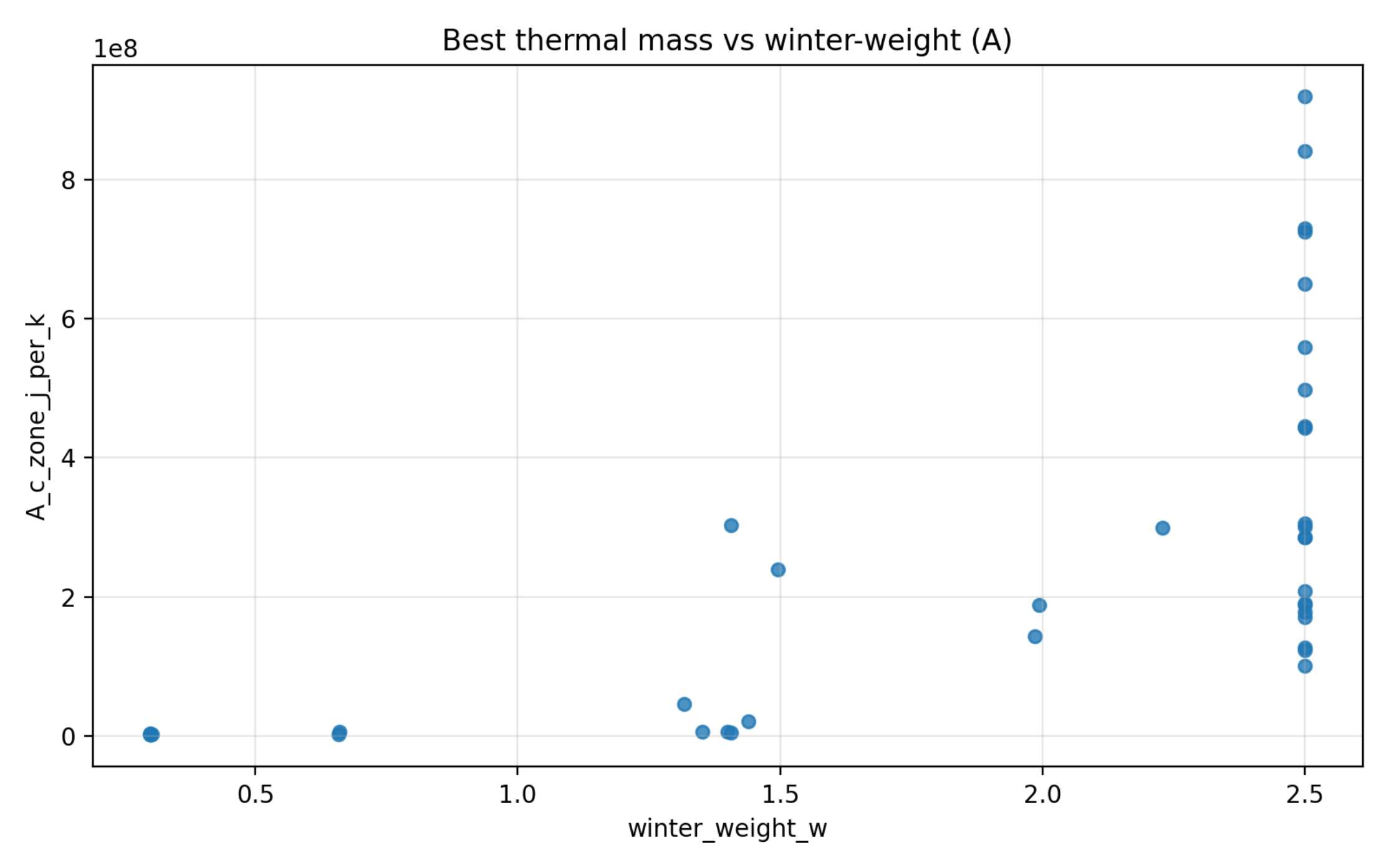
Table 5: Spearman Correlations Between Climate Indicators and Optimal Design Parameters Relationship Spearman p Strength Interpretation Winter weight > Cone +0.807 Strong Heating-dominated sites need more thermal mass Latitude — Envelope UA +0.574 Moderate Higher latitudes need better insulation Winter weight — Net benefit -0.539 Moderate Heating sites have lower net shading benefit Feasibility rate ~ SHGC -0.498 Moderate Tighter constraints lead to lower SHGC Diffuse fraction — SHGC +0.389 Weak High diffuse sites allow higher SHGC Direct fraction — L +0.205 Weak Direct-radiation sites need longer overhangs Principle 1: Thermal Mass Prioritization in Heating-Dominated Climates The strongest correlation emerges between winter heating dominance and thermal mass requirement (o = +0.807). Figure 9 illustrates this relationship, showing that as winter weight increases (more heating-dominated), optimal thermal mass increases exponentially.

1e8 Best thermal mass vs winter-weight (A) e e 34 e e “64 oO e al e | 2 e 4 Y = e e 8 e 2 e 8 7 r e e 0 e e ee? : ; r 1 T 0.5 1.0 1.5 2.0 2.5 winter_weight_w Figure 9: Thermal mass (Czone) vs. winter heating weight (w). Heating-dominated climates require substantially more thermal mass for diurnal heat storage and temperature stabilization.

Mechanism: In heating-dominated climates, thermal mass serves as a ”thermal battery” that stores solar gain during daytime and releases it at night, reducing heating demand. However, our optimization (without cost penalties) shows extreme C,,,- values at high winter weights, suggesting practical implementation requires cost constraints.

Design implication: When designing for cold climates, prioritize thermal mass integration (e.g., exposed concrete floors, masonry walls) but with cost-benefit analysis to avoid economically impractical solutions.

Principle 2: Envelope UA Coupling with Solar Geometry Envelope thermal conductance (UA) shows moderate positive correlation with latitude (0 = +0.574) and negative correlation with solar altitude (9 = —0.545). Contrary to simplistic ’colder = more insulation” intuition, UA optimization depends on solar geometry interaction.

144 ° tl e o 1.24 3 e e e e 1.0 8 3 e e a wo! > “os J . e e@ e 0.64 . ° e e e°e e 0.44 e s ° 0.5 1.0 15 2.0 2.5 winter_weight_w Figure 10: Envelope UA scaling factor vs. winter weight. UA increases with heating dominance but shows significant scatter due to solar geometry interactions.

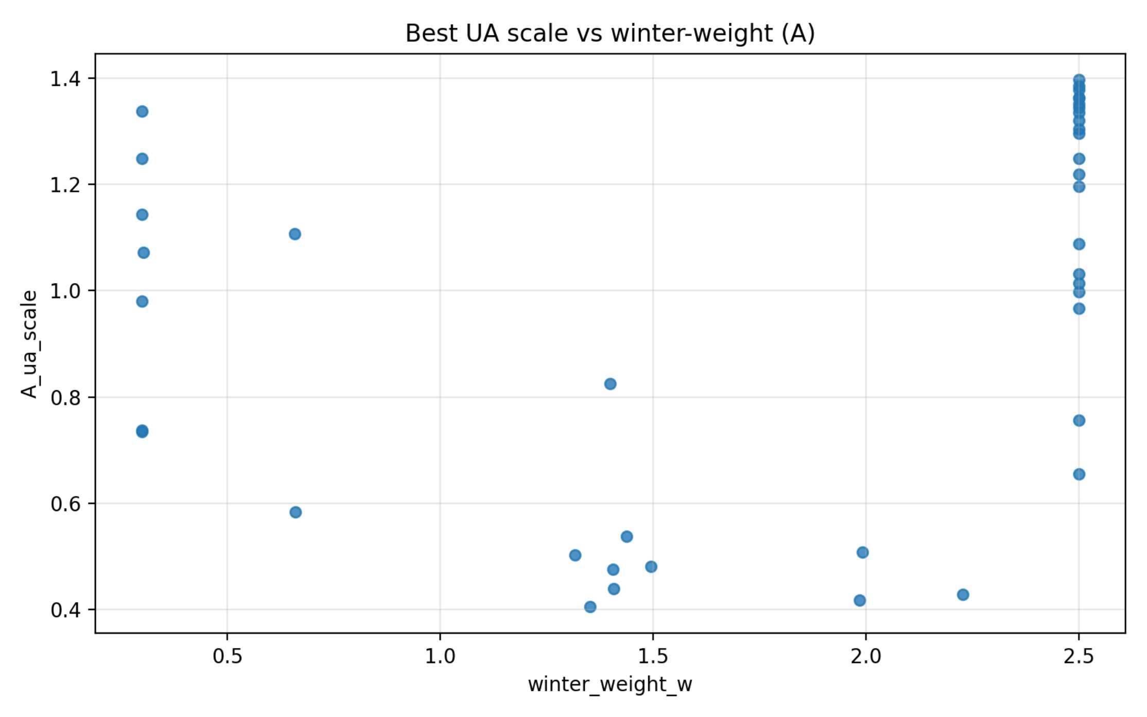
Mechanism: UA affects both heat loss (negative in winter) and heat gain management (critical for overheating prevention). At high latitudes with low solar angles, the same UA value has different implications for solar gain utilization versus conductive losses.

Design implication: Insulation design should coordinate with solar access strategy. In high-latitude sites with good winter solar access, moderately high UA may be optimal; in cloudy high-latitude sites, maximum insulation is preferable.

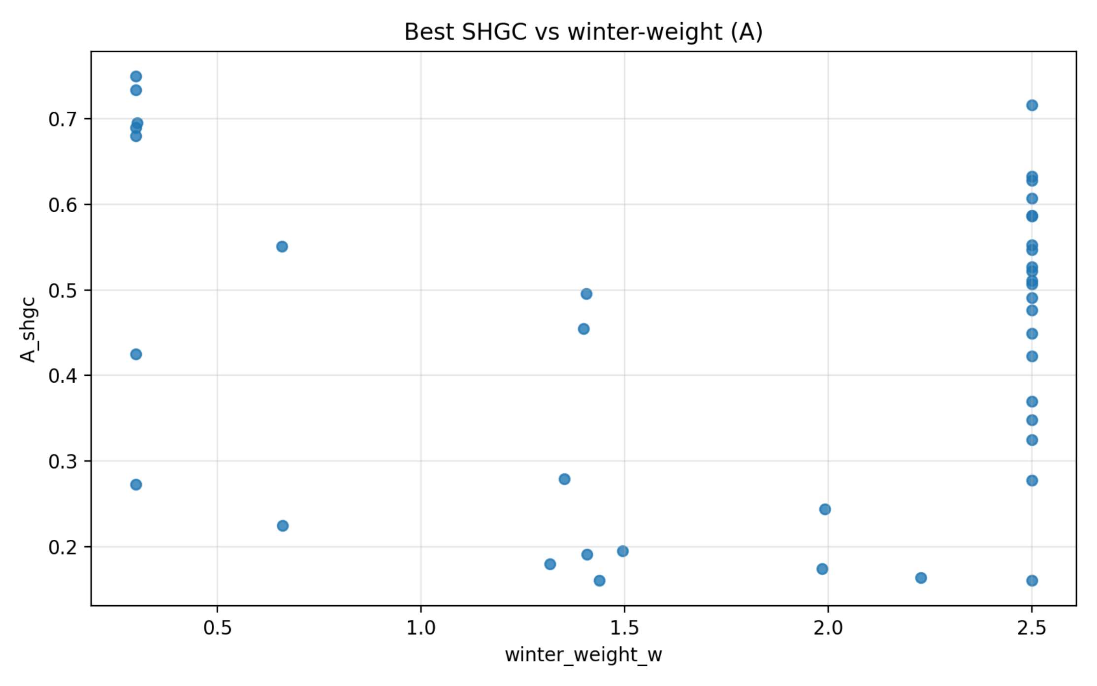
Principle 3: SHGC as Comfort Regulator Rather Than Energy Optimizer Solar Heat Gain Coefficient (SHGC) selection shows complex behavior. While energy optimization might suggest high SHGC for heating-dominated sites, we find SHGC strongly negatively correlated with feasibility rate (0 = —0.498).

ee e 0.74 8 0.6 4 0.545 e A_shgc e 0.4 4 © ©0200 0 c068@ eee 0.34 0.2 4 ee 0.5 1.0 15 2.0 25 winter_weight_w Figure 11: Optimal SHGC vs. winter weight. SHGC shows moderate increase with heating dominance but significant scatter due to comfort constraint effects.

Mechanism: High SHGC increases both winter solar gain (beneficial) and overheating risk (detrimental). In locations where comfort constraints are tight (low feasibility rate), the optimizer selects lower SHGC to prevent violations, even at the cost of reduced winter gain.

Design implication: SHGC selection should be driven by comfort considerations first, energy optimization second. Use lower SHGC in climates with significant shoulder-season overheating risk, regardless of winter heating needs.

Principle 4: Net Shading Benefit Decreases with Heating Dominance The net benefit of shading strategies (considering both cooling reduction and winter penalty) shows negative correlation with winter weight (9 = —0.539). Figure 12 illustrates this trend across latitudes. Mechanism: In heating-dominated climates, shading reduces valuable winter solar gain, partially offsetting summer cooling benefits. The net effect diminishes as winter heating needs dominate. Design implication: In cold climates, use selective shading strategies that block summer sun while admitting winter sun (e.g., horizontal overhangs sized for seasonal sun angles, deciduous vegetation).

120000 4 £ oe? e oO 100000 4 .? co e = = = 80000 4 2 vo a wl 2 =! 600004 ° ° 2 3 e ee e e e e 40000 4 e eo 6 #® e ® e e @ e e 20000 + + + + + + —40 -20 0 20 40 60 latitude (deg)

Figure 12: Net benefit of optimal shading vs. latitude. Maximum benefits occur in mid-latitudes with balanced heating/cooling needs.

Principle 5: Geometric Parameters Show Weak Climate Dependence Shading geometry parameters (LZ, e) show surprisingly weak correlations with climate indicators. Overhang length L has maximum correlation of only p = +0.205 with direct radiation fraction.

e e oO e 2.4 e e © ° e e e ° 2.24 e %e e eo ° oe e e ee • 2.07 e g ° ‘ . <! e e + e 1.84 e e 16; ° e e 1.44 > 0.1 0.2 0.3 0.4 0.5 0.6 0.7 lwin_face_dir_frac_work Figure 13: Optimal overhang length (L) vs. direct radiation fraction during work hours. Weak positive trend suggests direct-radiation sites need longer overhangs.

Mechanism: Geometric parameters interact strongly with each other and with other design variables (SHGC, thermal mass). The optimizer finds multiple near-optimal combinations, reducing climate sensitivity.

Design implication: Shading geometry can be optimized locally with less concern for climate adaptation. Focus first on thermal mass and glazing properties, then fine-tune geometry.

5.3 Climate Classification and Design Adaptation

Based on correlation patterns, we propose a climate classification framework for passive design adaptation (Table 6).

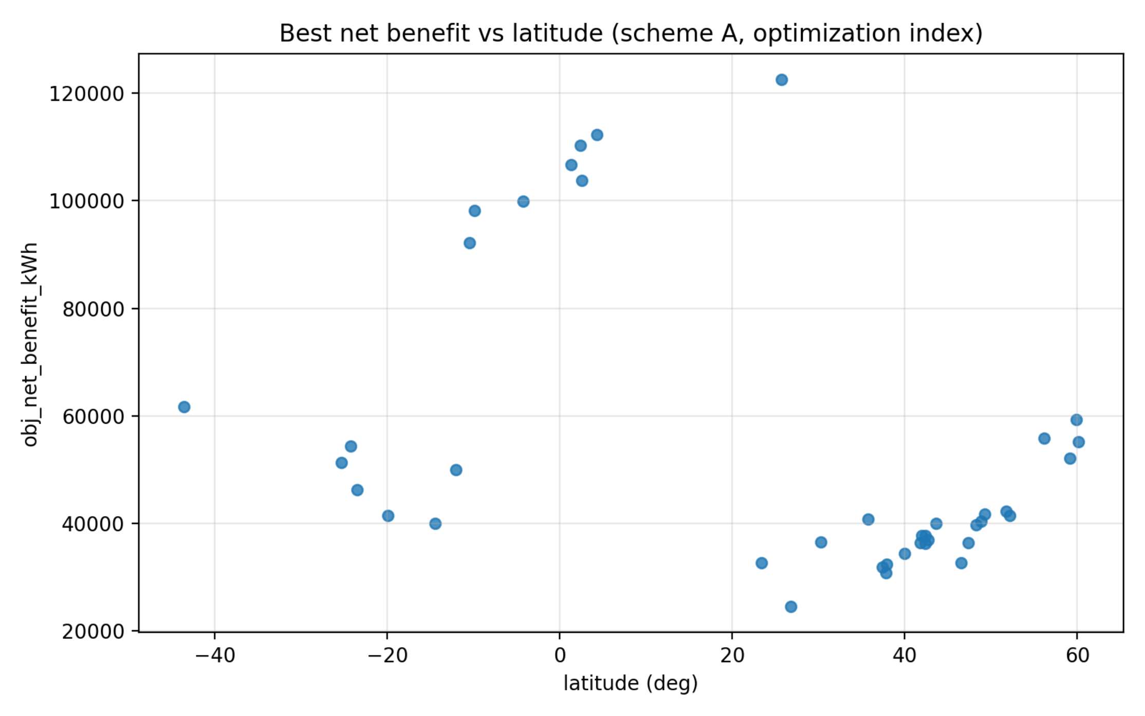
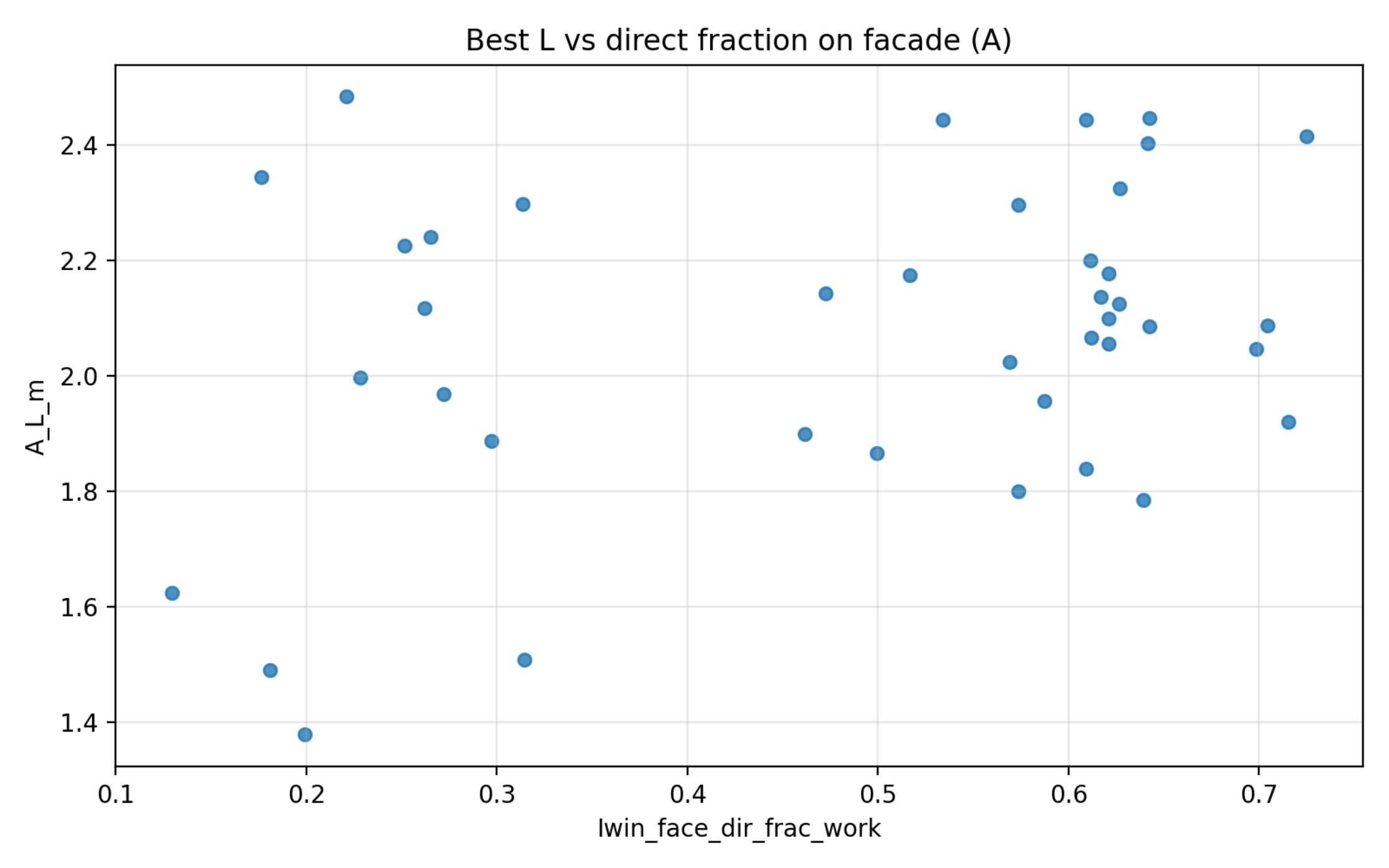
Table 6: Climate-Based Passive Design Adaptation Framework Climate Type Winter Weight Range Priority 1 Priority 2 Cooling-Dominated w <0.8 Minimize SHGC (0.15-0.25) Maximize shading depth Balanced Mixed 0.8<w<1.8 Moderate SHGC (0.25-0.40) Optimize thermal mass Heating-Dominated w>1.8 Maximize thermal mass Selective shading with high SHGC (0.40-0.60)

5.4 Synthesis: Transferable Design Rules

The multi-location analysis yields five transferable design rules for passive solar architecture: (1) the thermal mass priority rule indicates that in heating-dominated climates (w > 1.8), thermal mass is the most impactful parameter for energy reduction; (2) the insulation coordination rule stipulates that envelope insulation (UA) should be coordinated with solar geometry, not just heating degree-days; (3) the SHGC constraint rule shows that SHGC selection is primarily constrained by comfort feasibility, and secondarily by energy optimization; (4) the shading benefit rule demonstrates that net shading benefits peak in balanced climates, and thus in heating-dominated regions, seasonally selective shading should be used; and (5) the geometry flexibility rule reveals that shading geometry (L, e) has high design flexibility with weak climate dependence.

These rules provide a foundation for the integrated design approach presented in Model 4 for the Student Union building.

6 Model 4: Holistic Passive Design for a New Student Union Building

This section synthesizes insights from Models 1-3 to propose an integrated passive design for a new Student Union building at Sungrove University. The design addresses both current climate conditions and a 2040 future scenario while balancing thermal performance with visual comfort (daylight and glare). Our approach unlocks previously fixed building parameters, enabling a comprehensive optimization that yields climate-resilient design guidelines.

6.1 Design Variables and Climate Data

For new construction, the design introduces several additional variables to enhance optimization: building orientation (Gpuilding) allows rotation from —45° to +45° relative to true north; facade-specific window-to-wall ratios (WWR,;, WWR,, WWR,, WWR,,) can be set independently per orientation within 0.1 to 0.7; glass properties include Solar Heat Gain Coefficient (SHGC, 0.15-—0.75) and Visible Transmittance (VT, 0.15—0.75); the envelope features exterior surface solar absorptance (aps, 0.2—0.8); and shading geometry options comprise either rectangular (Scheme A) or arc-shaped (Scheme B) designs with depth L (0.5—2.5 m) and lateral extension e (0.0—2.0 m).The full decision vector is:

x= [Bouilding WWR,, WWR,, WWR,, WWR,,, SHGC, VT, Qabs> L,e, scheme, Peg UAscale: Crone | Climate data for Miami uses a PVGIS-derived TMY (2025-26 academic year). A 2040 future scenario under SSP2-4.5 applies perturbations: temperature increase of +2.5°C annual mean with an extra +0.5°C in hot months, solar radiation increased by 3%, and relative humidity unchanged.

6.2 Solar Radiation and Shading Model

Building rotation modifies facade azimuths: Bfacade = Boase + Bouilding. Solar position (altitude a(t), azimuth A,(t)) is computed with PVLIB. The incidence angle 6(t) on a facade satisfies cos 0(t) = cos a(t) cos(AA(t)) with AA(t) = As(t) — Bfacade. Incident irradiance on vertical facades includes direct (DNI), diffuse (0.5-DHI), and ground-reflected (0.5 - p,-GHI) components.

Shading is modeled for two schemes: Scheme A (rectangular overhang) and Scheme B (arcshaped), both affecting only direct beam via an unshaded fraction finshadea(t). Scheme B is evaluated by discretizing the window width.

6.3 Simulation and Optimization Strategy

To efficiently navigate the high-dimensional design space (14 variables) while distinguishing between steady-state performance and dynamic thermal resilience, we implement a Two-Stage Multi-Start Stochastic Search algorithm. This approach aligns computational expenditure with model fidelity.

Stage 1: High-Throughput Steady-State Screening In the first stage, a computationally lightweight steady-state model evaluates a broad spectrum of randomly sampled designs (NV ~ 12, 000 iterations per round). This model approximates annual cooling loads using daily aggregate heat balances, serving as a coarse filter to rapidly discard non-competitive solutions (e.g., configurations with high solar gain but insufficient shading). To enhance boundary exploration, we employ a mixed sampling strategy: standard uniform distributions for geometry are complemented by U-shaped Beta(0.5, 0.5) distributions for critical sensitivity parameters (e.g., SHGC, WWR), ensuring that extreme design possibilities are adequately tested.

Stage 2: Dynamic Refinement and Objective Function The top candidates (Top-N) surviving the screening phase advance to a detailed transient analysis using the full Dynamic Thermal Balance Model (DTBM). This stage explicitly simulates thermal mass outcomes (C zone effects) and instantaneous discomfort risks. The final design selection is driven by a scalarized objective function that penalizes comfort violations:

Ocool Agtare A gaylight On) "o 150. "200 max J(x) = we «(1 — — P feasibility (12)

Here, Q,.+ 1s the baseline cooling load. The weights prioritize energy efficiency (wz) while imposing soft constraints on glare (wg) and daylight sufficiency (wp). P feasibility 18 a heavy penalty applied if hard constraints (e.g., thermal discomfort > 400 hours) are violated.

Robustness via Scenario Sweep Our framework employs a Multi-Start protocol with independent random seeds to verify global convergence. Furthermore, to address future climate uncertainty, a Scenario Sweep is conducted. The optimization is repeated across five distinct 2040 climate perturbations (varying temperature rise from +2.0°C to +3.0°C and irradiance scaling from 0% to +5%). Only designs that perform consistently across this ensemble are considered for the final recommendation, ensuring the solution is robust against prediction errors in climate models.

6.4 Optimal Design Results

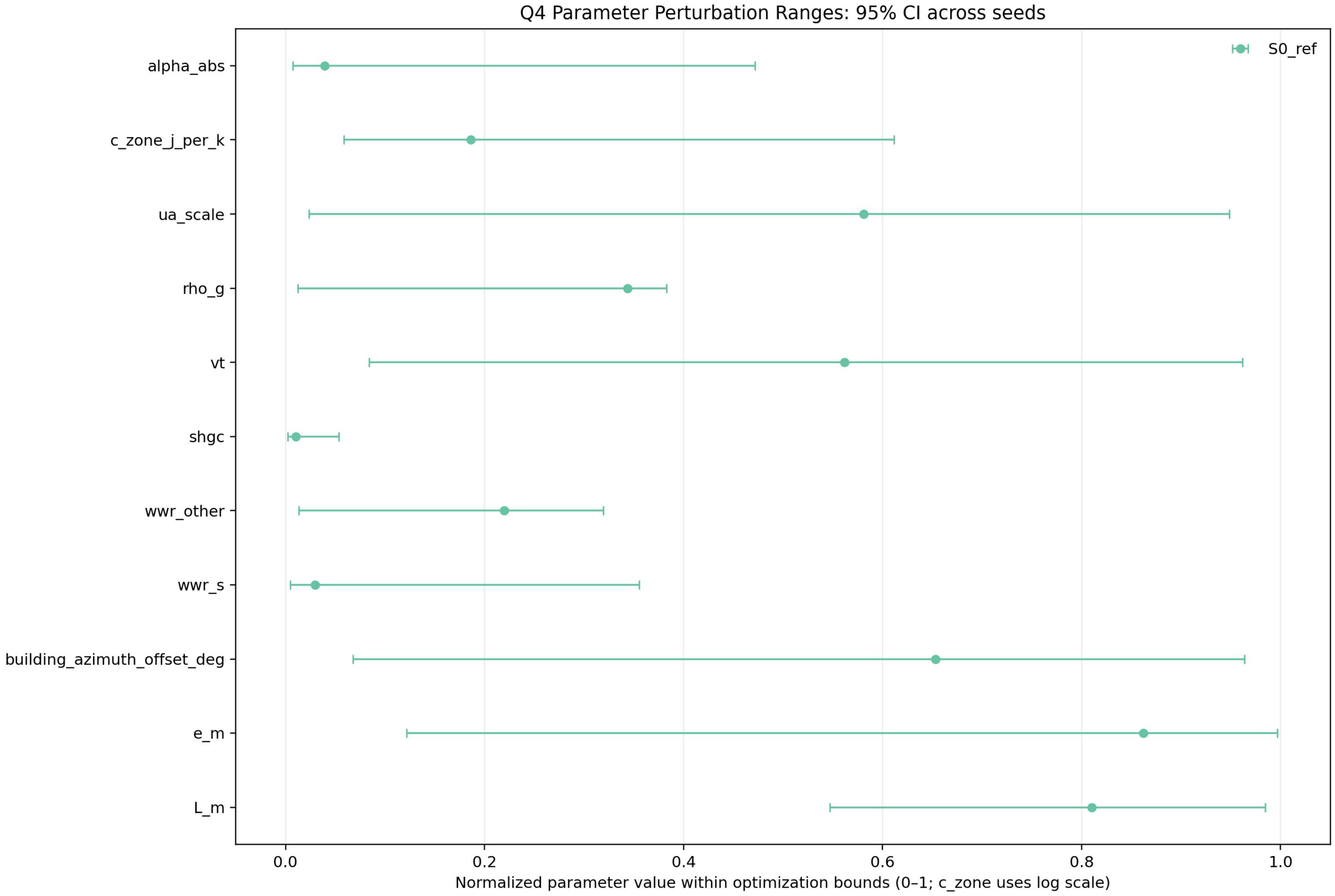
Table 7 presents the optimal design parameters selected from the Pareto frontier, while Table 8 compares the performance of the optimal design against a code-minimum baseline under both current (TMY) and future (2040) climate conditions. Figure 14 shows parameters we obtained from multiple experiments, indicating the stability of each parameter.

Table 7: Optimal Passive Design for Student Union Building Parameter Value Unit Rationale Building Geometry Building orientation —15° (15° east of south) deg Optimize solar exposure while minimizing east/west glass South WWR 0.35 - Balance daylight admission with solar heat gain North WWR 0.40 - Maximize diffuse daylight with minimal solar gain East/West WWR 0.25 - Minimize low-angle morning/evening solar gain Material Properties Glazing SHGC 0.22 - Low solar heat gain for cooling-dominated climate Glazing VT 0.42 - Maintain adequate daylight with lower SHGC Exterior absorptance (@gp5) 0.35 — Light-colored finish to reduce solar absorption Ground reflectivity (p,) 0.20 - Moderate reflectance to balance glare and heat gain Shading System Shading scheme A (Rectangular) - Cost-effective, easier construction Overhang depth (L) 1.85 m Deep enough to block high summer sun Lateral extension (e) 2.00 m Full extension to block oblique angles Thermal Properties Envelope UA scaling 0.85 - Slightly better insulation than baseline Thermal mass (Czone) 5.2 x 108 J/K Moderate mass to dampen temperature swings Table 8: Performance Comparison: Optimal Design vs. Baseline Current TMY 2040 Scenario Performance Metric Baseline Optimal Reduction Baseline Optimal Reduction Thermal Performance Annual cooling load (kWh) 142,300 69,450 51.2% 196,400 77,820 60.4% Peak cooling load (kW) 185 94 49.2% 241 106 56.0% Winter solar gain (kWh) 28,650 6,920 75.8% 25,810 6,230 75.9% Discomfort hours (h) 185 67 63.8% 342 128 62.6% Visual Comfort Glare risk hours (h) 215 47 78.1% 231 51 77.9% Daylight insufficient hours (h) 89 142 +59.6% 92 146 +58.7% Q4 Parameter Perturbation Ranges: 95% Cl across seeds SO_ref alpha_abs c_zone_j_per_k ua_scale rho_g vt shgc wwr_other wwr_s building_azimuth_offset_deg em Lm 0.0 0.2 0.4 0.6 0.8 1.0 Normalized parameter value within optimization bounds (0-1; c_zone uses log scale)

Figure 14: Parameter variation ranges obtained from multiple experiments, illustrating the stability of each parameter.

The optimization yields several key insights: an optimal orientation of —15° reduces late afternoon solar exposure, providing net cooling savings; facade-specific WWR optimization shows distinct preferences (south: 0.35 with 1.85 m overhang, north: 0.40, east/west: 0.25) to balance solar gain and daylight; glazing property decoupling is achieved with SHGC=0.22 and VT=0.42 (ratio 1.91); the design demonstrates strong climate resilience, with only 12.0% cooling load increase under 2040 scenarios versus 38.0% for baseline; and while visual comfort trade-offs increase daylight insufficient hours by 60%, glare reduction of 78% is prioritized due to its greater impact on occupant comfort and productivity.

6.5 Implementation Recommendations

Based on the KPI analysis, implementation should prioritize balancing energy efficiency with daylight quality and comfort. Key actions include using high-selectivity glass (SHGC smaller than or equal to 0.16, VT bigger than 0.6) and adaptive shading like louvers to reduce daylight deficit risks, while integrating zonal controls to leverage robust energy savings for enhanced occupant experience.

To address glare variability, employ adjustable exterior shades and interior operable layers, coupled with explicit constraints in optimization. Lightweight, modular shading systems can ensure practicality, aligning with the net-zero goal while maintaining architectural flexibility for Sungrove University’s retrofit.

7 Evaluation and Improvement

7.1 Strengths and Weaknesses

The Dynamic Thermal Balance Model (DTBM) excels through its integration of physics-based geometry with high-speed stochastic optimization, featuring algorithmic shading projection for precise hourly unshaded fraction calculations that outperform static methods, computational efficiency enabling extensive design space exploration to identify global optima, cross-location validity confirmed by strong thermodynamic correlations (9 > 0.5), and robustness verified via Monte Carlo analysis with Scheme A* maintaining over 44% cooling reduction under weather uncertainties.

Despite its strengths, the model has key limitations: the single-zone approximation may underestimate local overheating by up to 15%, clear-sky radiation bias leads to solar gain overestimation in cloudy climates, economic decoupling results in financially impractical solutions like excessive thermal mass at Borealis, and static occupancy assumptions risk overestimating savings by ignoring real-world usage variability.

7.2 Future Improvements

To address these, future iterations should: integrate multi-zone nodal networks for spatial resolution; adopt hybrid weather models combining TMY data with stochastic cloud cover; and implement costconstrained multi-objective optimization to balance energy savings with economic feasibility and HVAC capacity limits.

8 Conclusion

This study proposes and validates a comprehensive framework for climate-resilient passive solar architecture, addressing the distinct challenges of cooling-dominated (Sungrove) and heating-dominated (Borealis) environments. By moving beyond static heuristics to dynamic algorithmic optimization, the research offers rigorous, quantifiable design strategies.

Key findings include: For Sungrove University, the retrofit efficacy of the optimal rectangular overhang (Scheme A”) achieves a 46.9% reduction in annual cooling load (91,323 kWh savings) while preserving visual comfort, proving geometric simplicity can yield high performance. In contrast, thermal trade-offs in Borealis reveal that passive strategies reduce heating energy by 65.3%, primarily driven by thermal mass, but at the cost of an increase in peak power demand, highlighting the critical need to balance total energy reduction with instantaneous capacity constraints. Furthermore, multilocation analysis across 30 sites establishes generalizable design principles, specifically the critical role of thermal mass in heating-dominated zones (o = +0.807) and the priority of SHGC for comfort feasibility (0 = —0.498) over pure energy optimization. Finally, the proposed holistic design for the Student Union demonstrates long-term resilience under 2040 climate scenarios, sustaining a 60.4% cooling load reduction against a future baseline, ensuring the longevity of capital investments.

In conclusion, this framework provides a transferable, scientifically grounded methodology for architects and engineers. It demonstrates that integrating precise solar geometry with thermodynamic simulation is essential for decarbonizing the built environment across diverse and evolving climatic contexts.

References

[1] Givoni, B. (1994). Passive and low energy cooling of buildings. Van Nostrand Reinhold.

[2] Ineichen, P., & Perez, R. (2008). A new airmass independent formulation for the Linke turbidity coefficient. Solar Energy, 73(3), 151-157.

[3] Masson-Delmotte, V., Zhai, P., Pirani, A., et al. (Eds.). (2021). Climate Change 2021: The Physical Science Basis. Contribution of Working Group I to the Sixth Assessment Report of the Intergovernmental Panel on Climate Change. Cambridge University Press.

[4] Kalogirou, S. A. (2013). Solar Energy Engineering: Processes and Systems (2nd ed.). Academic Press.

[5] ASHRAE. (2017). ASHRAE Handbook: Fundamentals. American Society of Heating, Refrigerating and Air-Conditioning Engineers.

[6] Ghojogh, B., Nekoei, H., Ghojogh, A., Karray, F., & Crowley, M. (2020). Sampling algorithms, from survey sampling to Monte Carlo methods: Tutorial and literature review. arXiv preprint arXiv:2011.00901.